Over the course of lab weeks 7 and 8, our class looked at problems of reproducibility and replicability in geography. We focused on a paper titled “Vulnerability Modeling for Sub-saharan Africa: an Operationalized Approach in Malawi” published by Malcomb, Weaver, and Krakowka (Malcomb 2014). We read through the paper and tried to recreate their findings from the information the paper provided in the methods section. We ran into some immediate problems with the idea of a vulnerability analysis. Jochen Hinkel argues that there is not real way to measure vulnerability because there is so much spatial heterogenity in vulnerability analysis and the real impacts of vulnerability cannot be easily measured nor should they be confused with measurements of harm (Hinkel 2011). This point speaks to a greater issue about the challenges of reproducing qualitative data. Malcomb et al. determined that vulnerability could be described in terms of resilience based on adaptive capacity which they decided was determined by a household’s assets and access to resources. The factors that malcomb et al. used to determine adaptive capacity and thus vulnerability were determined from surveys of people living in Malawi.
With factors determined, Malcomb et al. used data from DHS surveys and clusters years 2004 and 2010 to assess assets at the household level. We were able to gain access to this data and used in our reproduction of the results. However, we ran into an issue with access to data because in addition to using the DHS surveys, Malcomb et al. used FEWSNET 2005 data to determine livlihood sensitivity which we did not have access to. FEWSNET 2005 data accounted for 20% of the final vulnerability anaylsis, so even if we did everything else that Malcomb et al. did, our results will only ever be 80% complete.
We obtained the same data as Malcob et al. that we could access: DHS surveys and cluster points estimated risk for Flood Hazard and exposition to drought events from UNEP global risk platform GADM version 2.8 boundaries for Malawi FEWSNET livelihood zones
We used the PostGIS extenstion of PostGresSQl as our GIS platform and QGIS to visulize the results
Malcomb et al. assigned a vulnerability score from 1-5 to each household based on the vulnerability indicators chosen for the study. The indicators from the DHS data was categorized uder adaptive capacity which was further broken down into assest and access. Malcomb et al. determined that assests and access factors each contributed 20% to the over all vulnerability (40% together). 20% of the vulnerability was attributed to livelihood sensitivity (FEWSNET data) that we did not have access to. And the final 40% was attributed to physical exposure which was subdivided into “Estimated Risk for Flood Hazard” and “Exposition to Drought Events” Each of which were given 20% contribution to vulnerability. The data for the phyiscal exposure came from the UNEP Global Risk Data Platform (GRID). We used
Our first step in reproducing Malcomb et al.’s findings was to assign a vulnerability score (1-5) to each household for each
indicator in the adaptability analysis. We did this step as a class each taking on one asset to classify. Complete SQL file for the
class process: SQL This file also includes the process for deleting
missing data and joining the information from tables together.
To classify the assests on a scale of 1-5, we used the ntile function, but ntile cannot account for indicators that were given the same score, so scores needed to be converted first to a percent rank because percent rank allows ntile to account for ties in the indicator scores. Here is an example of an SQL query that demonstrates converting the survey entries from the number of sick people per household into a vulnerabilty score:
Step 1: add a column
ALTER TABLE dhshh ADD COLUMN sick REAL;
Step 2: udpate table to make scores a percent rank
UPDATE dhshh set sick=pctr from
(SELECT hhid as shhid, percent_rank() OVER(ORDER BY hv248 desc) * 4 + 1 as pctr FROM dhshh ) as subq
where hhid=shhid;
Step 3: give score 1-5 with ntile function
SELECT hhid, ta_id,
NTILE(5) OVER(
	ORDER BY hv248
) AS num_sick,
An important thing to note: some indicators need to be assigned scores in order descending because a higher number indicates a more vulnerable state. In the case of sick people per household, sickness indicates more vulnerability. More sick people = lower score. In other cases, such as livestock per household where more livestock means more adaptability More livestock = higher score.
our class ran into a reproducability problem with indicators that were entered as true or false. For example, having a radio, or electricty was entered as 1 for true, 0 for false in the survey. Malcomb et al. did not describe their process for for converting true/false answers into a 1-5 score. In our anaylsis we decided to give true answers a value of 5 and false a value of 1, but we are aware that this distorts our results by limiting these indicators to being either extremely good or extremely bad.
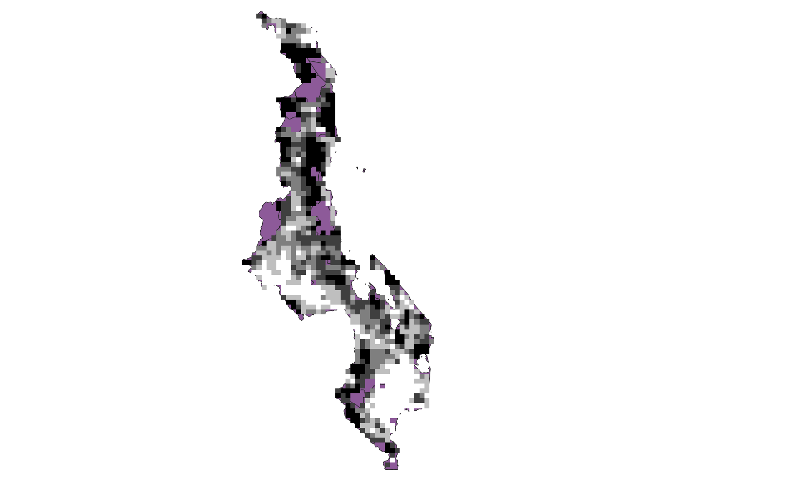
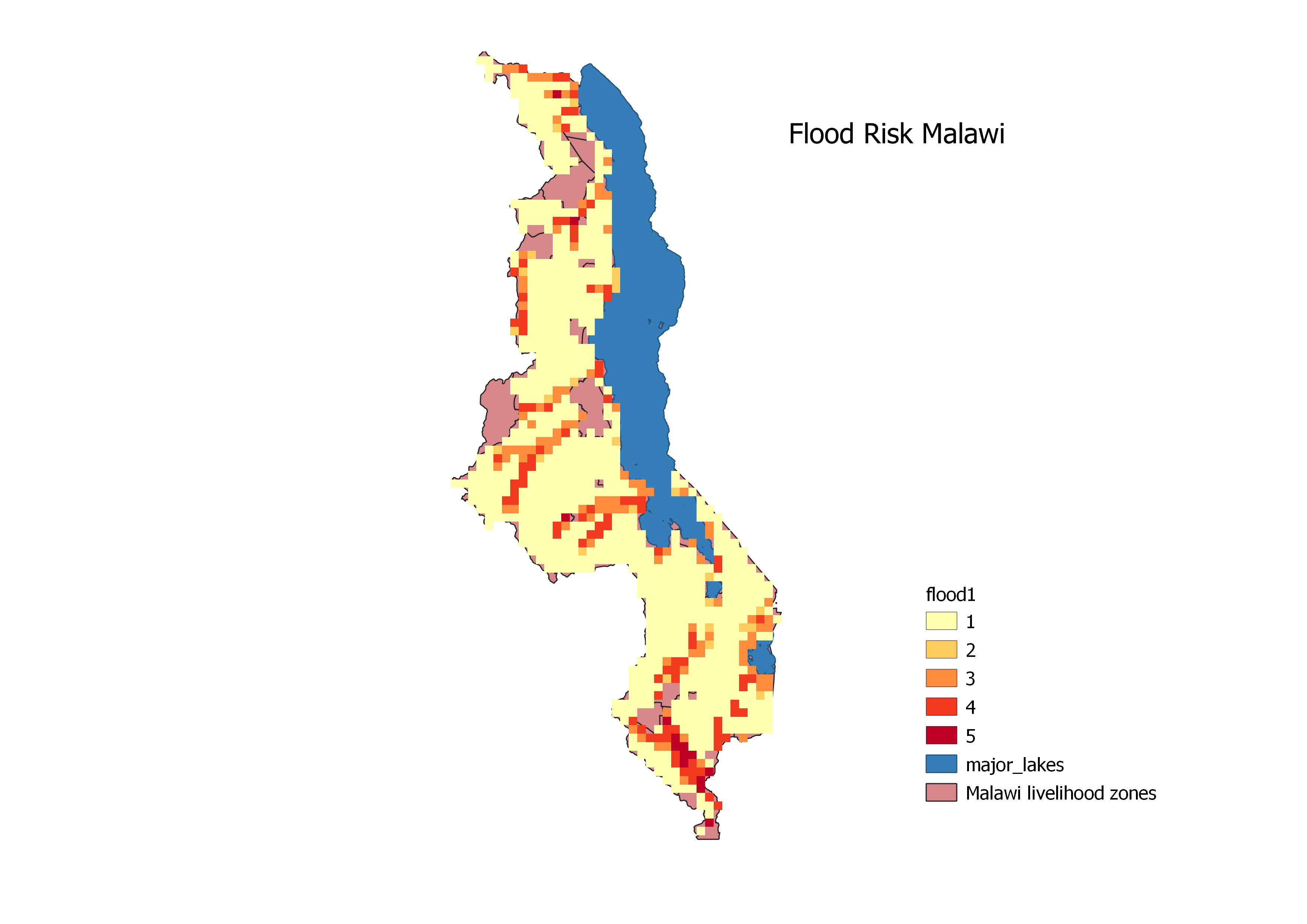
Next indicator scores were multiplied by their weights and summed to give a score for each household. Going into the next lab, Professor Holler provided this model for the following analysis vulnerabilitymodel This model went through the steps of (1) extracting the vulnerability scores from the “CapacityValue” and making it into the “capacity” layer. (2) giving our map an extent by clipping “capacity” to the extent of the “livelihoodZones” layer. “livelihoodZones” is the extent of Malawi’s political boundaries minus the lake that borders the country. (3) Rasterize the “flood”, “drought” and “capacity” layers so that we can work with them as raster data. “flood” and “drought” layers were downloaded from the GRID UNEP site https://preview.grid.unep.ch/index.php?preview=data&lang=eng (4) drought and flood layers were masked to the “Capacity Grid” so that there will be no data in these layer for cells in which there is no data on the capacity layer. Next we used raster functions in QGIS to give the “floodclip” and the “droughtclip” layers scores from 1-5 based the severvity of their inputs. For “droughtclip” we added r.quantile that gives its output in html file form which we saved as a txt file then used in the r.rcode function with the drought to create classifed layers. This is the output of that function layed over the Livelihoodzones layer to contextualize the extent of Malawi: droughtoutput notice that there are rather large areas of no data in the drought layer. the “floodclip” layer already has only 5 classifications after rasterization but the range is 0-4. To make this layer consistant with the drought and capacity layers we used a raster calculator: “floodclip” + 1 and to shift the range to 1-5. The output of the flood layer looks like this floodoutput notice again the large areas of no data.
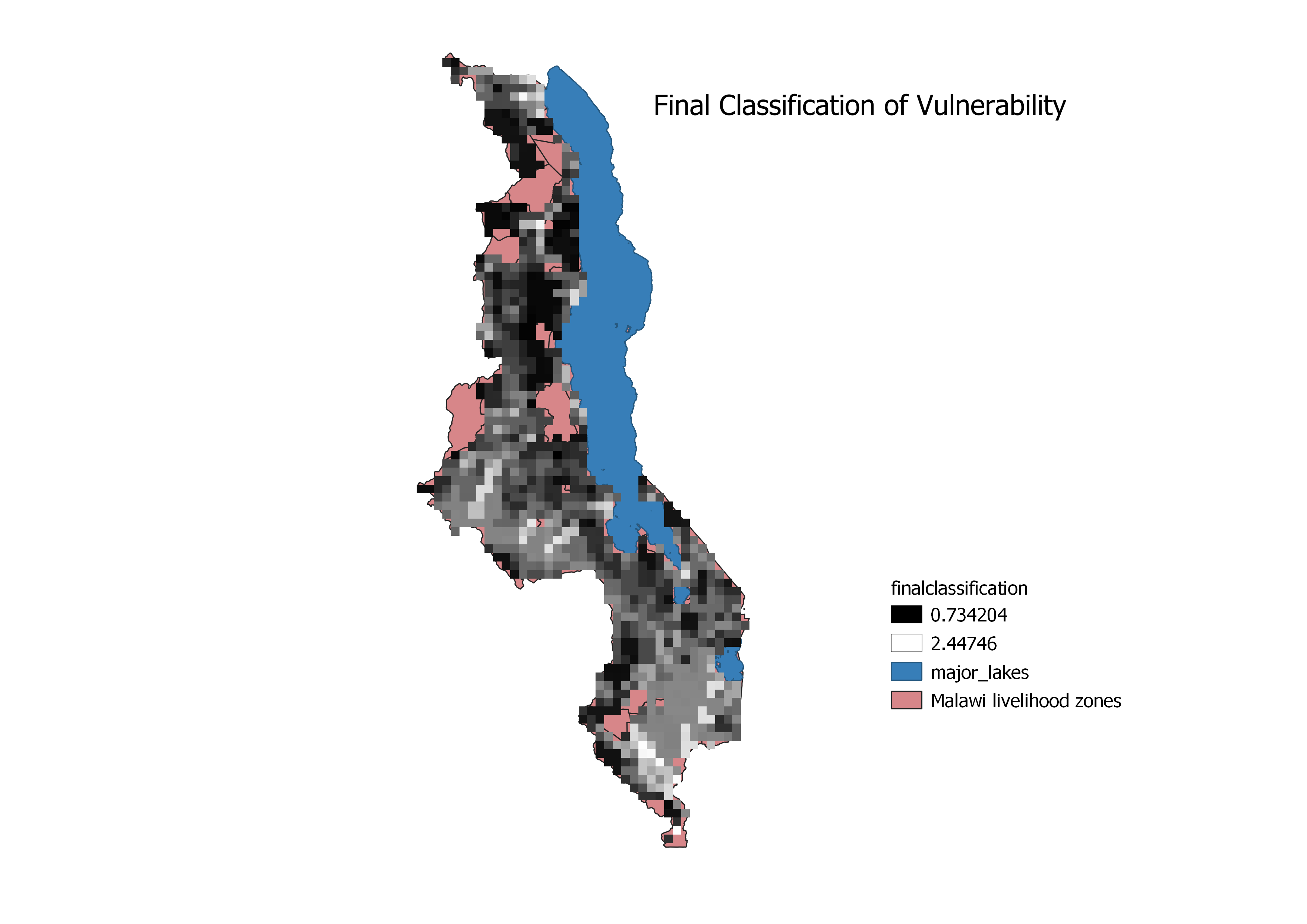
Next, to combine “capacityGrid”, “Floodoutput” and “droughtoutput” we used raster calculator to weight each given Malcomb et al.’s determined weights (40%, 20%, 20%) and added them together: ((2-“CapacityGrid”).4)+(“Floodoutput”.2)+ (“Droughtoutput”*.2)= final classification
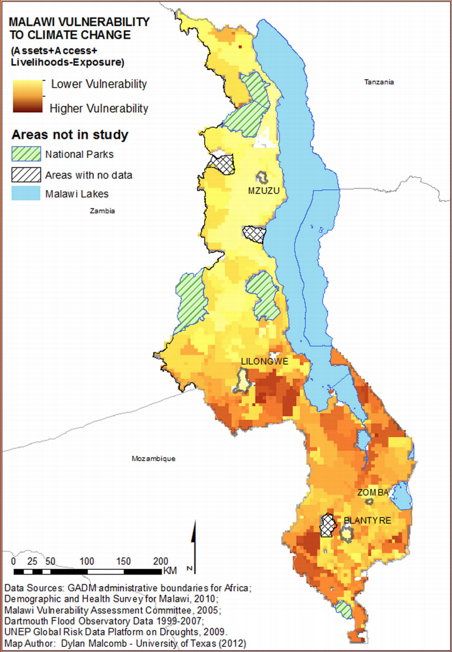
This final calssification visual is our reproduction of Malcomb et al.’s vulnerability assesmenet. Comparing our results to theirs, Malcomb Vulnerability there are some noticeable differences. Malcomb et al.’s map is at a finer resolution than ours because we used the drought layer to define the resolution for the flood layer because they were initally at different resolutions. Malcomb et al. did not state what their resolution was but we can assume that they used the flood layer to define their resolution. To overcome this error in reproducibility, we adjusted our model to allow the user to define the resolution model version 2 . We added the input “resolution” and a function to warp(reproject) the flood layer. “resolution” is an algorithm that allows the user to define the cell size. This issue with the cell size could have been easily avoided if Malcomb et al. had included the model as part of thier publication.
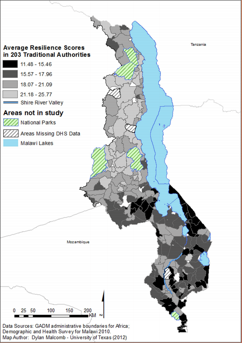
Aside from the lack of access to some of the data, we found some difficulties in reproducing the study because of a lack of explicit information about the methods. Malcomb et al. could make their study more reproducible by including their model with their methods. including a model would clear up the uncertainty about how they clipped the extenst of their data, what resolution they used, how they classified entries that were entered as true or false. For the replicability of the study they could also include a more in depth discussion of how they determined the indicators for vulnerability and whether those indicators would be applicable to another place. Finally, Malcomb et al. needs to include discussion about the sources of uncertainty. To protect the privacy of participants in the survey a buffer was placed around each survey point- a 5km radius for each point in a rural area and a 2km radius for each in an urban area. Then the survey point was randomly placed in that buffer zone so that the exact location of the survey was obscured. The source of error came in that Malcomb et al. analyzed resilience based on traditional authorities (TAs) shown on this map: Resilience TAs TAs are smaller politcal distinctions than districts, but in the survey data the district location was smallest political authority given for households. This means that survey points could be assigned to different TAs, but not different districts. this is a source of error for the analysis on TAs.
Resources: Malcomb, Dylan W., Elizabeth A. Weaver, and Amy Richmond Krakowka. “Vulnerability Modeling for Sub-Saharan Africa: An Operationalized Approach in Malawi.” Applied Geography 48 (March 1, 2014): 17–30. https://doi.org/10.1016/j.apgeog.2014.01.004. Hinkel, Jochen. “‘Indicators of Vulnerability and Adaptive Capacity’: Towards a Clarification of the Science–Policy Interface.” Global Environmental Change 21, no. 1 (February 1, 2011): 198–208. https://doi.org/10.1016/j.gloenvcha.2010.08.002.