week 3 lab

Introduction

The purpose of this lab was to learn how to use the tools in SAGA version 6.2 and SRTM and ASTER data to do a stream flow analysis for the area around mnt. Kilimanjaro.

Process

step 1: Download and import 2 DEM tiles of ASTER data collected by NASA and the Japanese Space System from the Earth Data Search website. https://lpdaac.usgs.gov/products/astgtmv003/ Users can download both the elevation and number files here. The granules that I downloaded were: ASTGTMV003_S03E037 and ASTGTMV003_S04E037

After importing the DEMs into the saga they will look like this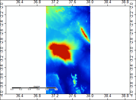

The DEMs need to be mosaiced together to create one seemless DEM. The Mosaicking tool lives under Grid> gridding> Mosaicking Use the Nearest Neighbor parameter to execute the tool. After the DEMS have been mosaicked they will look like this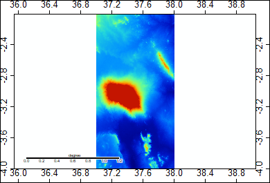

Step 2: The DEMs are now mosaicked together, but they are in WGS84. We need to reproject into World Mercator. to do this go to the projection tab under tools the to Proj.4 then to UTM projection (Grid). The »source is now the layer that was created from the DEMs that we mosaicked together. execute this step. Now the layers will be in World Mercator.

Step 3: To create a hillshade, go to the tools and under the Terrain Analysis tab go to Lighting, visibility then to Analytical Hillshading. The source is the Mosaicked DEM. Keep all other parameters in default. The output will look like this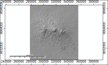

Step 4: Before we can do a hyrdological analysis, we have to identify the “sinks” in the landscape and remove them. This is a two step process. To detect the sinks in the elevation model go to the Terrain analysis tab under tools then to preprocessing then to Sink Drainage Route Dectection. The source is the mosaic. Keep all other parameters in default. The output will look like this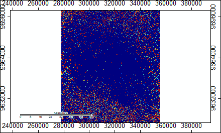

Step 5: Next we can remove the sinks using the previous layer we just created so that the sinks won’t cause errors in analysis later on. To remove the sinks go to the Terrain Analysis tab under the tools then to preprocessing and to sink removal. Use the Mosaic as the source and the sink Route layer made in the previous step as the Sink Route. Create the preprocessed DEM. It will look like this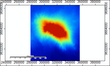

Step 6: Next to calcualte Flow accumulation go to terrain analysis under tools then to hydrology then to flow accumulation (top- Down) Use the Sink filled DEM for the elevation and the sink routes made in step 4 for the Sink Routes. Create the Flow accumulation layer and it will look like this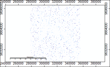

Step 7: The final step is to create the channel networks to determine where there are streams. Go to the terrain anaylsis under tools and to channels then to channel network. Again use the sink filled DEM for the elevation. Create the Channel network, the Channel Route, and the Channel Network (shapes) When you crteate this layer it will look like this.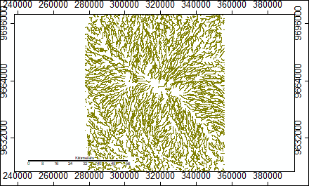

Lab 4

Introduction

For lab 4, we looked at the same study area but used a batch procress to run data to do hydrological analysis. We then used this batch process to run data from ASTER (same granules as lab3) as we did in the first lab and SRTM data collected by NASA at 1 arc second on the same area of mnt. Kilimanjaro. SRTM Elevation can be found here: https://lpdaac.usgs.gov/products/srtmgl1v003/ and the SRTM number files can be found here: https://lpdaac.usgs.gov/products/srtmgl1nv003/ The granules I used were: S03E037 and S04E037

The purpose of this lab was to evaluate level of error and uncertainty that there is in creating a stream flow analysis using this process.

Process

The batch process for the hydrological anaylsis of ASTER data looks like this ASTER Batch Process The batch process for the same analysis with SRTM data looks like this SRTM Batch Process Notice that the only difference between the two models are the prefix names and the file locations of the data.

Batch processes allow the user to run multiple data sets through the same anaylsis without having to run each tool individually in SAGA. This was useful for this lab because we could easily run the same process on two data sources.

The user can also run Number files for the study area through the first two steps of the batch procress so that the user will have a mosaicked and reprojected map of the number file. The number file has a code that allows the user to see where the data for each cell was drawn from in the procress of creating the elevation data. Using this number file the user can evaluate the prevalance of uncertainty and what sources were used to fill those gaps.

Once the user has the number file, they can reclassify it to show each source. an example of what it looks like for the ASTER data can seen here 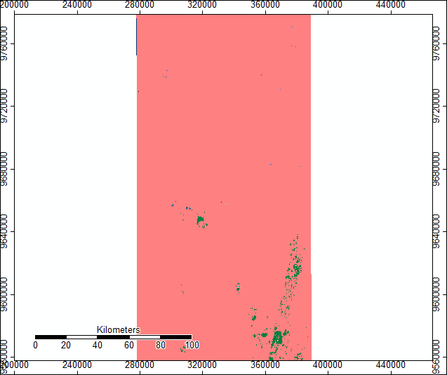a legend to interpret that can be found here

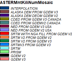
One can see using the number file and the legend that most of the data was GDEM V3, but that a large portion also shown in green is SRTM V2 from GDEM V3.

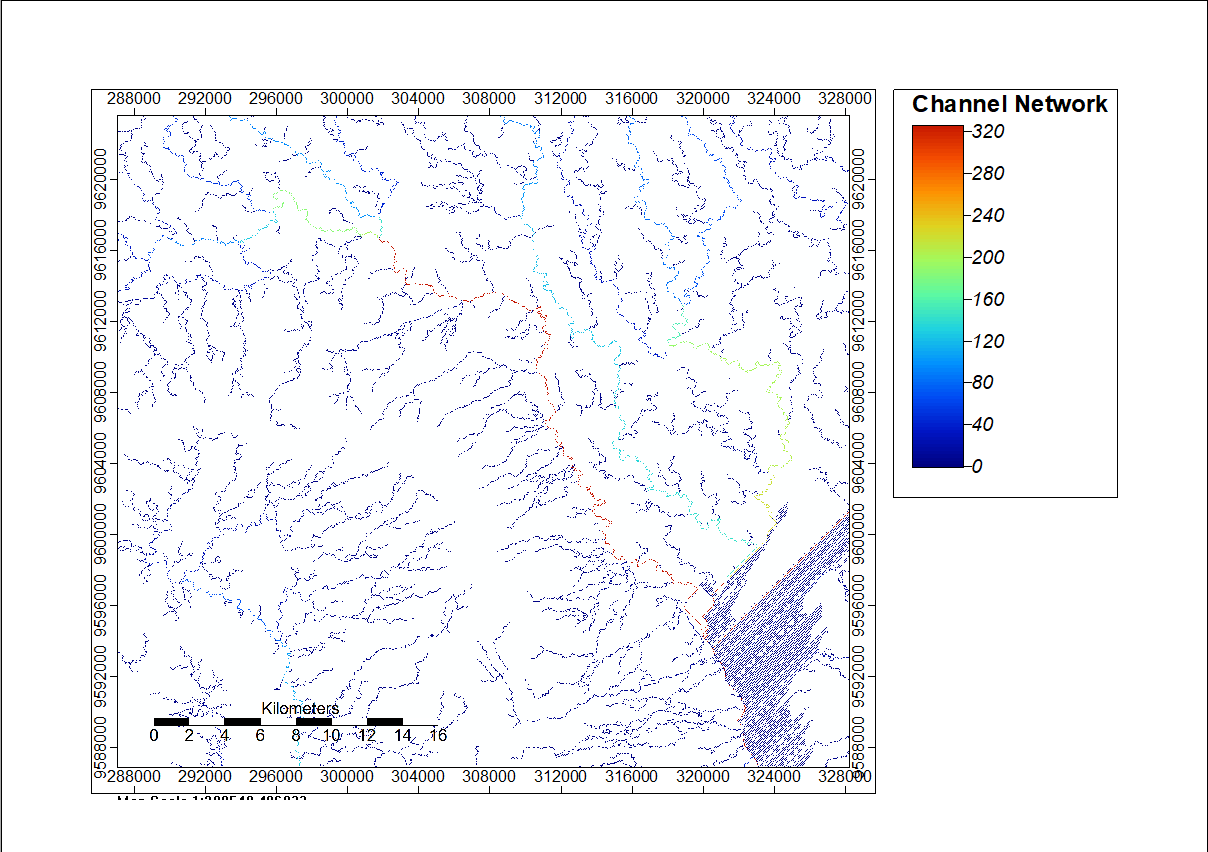
Channel network maps were the output of running the full batch process on the SRTM and ASTER DEM files: Here is a side by side comparison of a section of the the channel networks outputs for SRTM and ASTER.

ASTER

SRTM

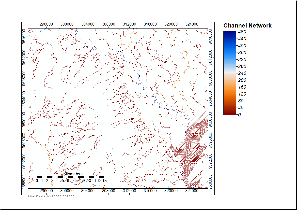
It is difficult to see any remarkable differences between the outputs of these two maps. However, the differences in two data sets cause there to be differences in the outputs which is a source of error for our anaylsis. To evaluate how DEM files created from SRTM and ASTER data differ we ran the grid difference tool that can be found under the Grid the calculus tabs in SAGA.I subtracted my ASTER- STRM to see the variance in elevation data between them. The resulting map looks like this 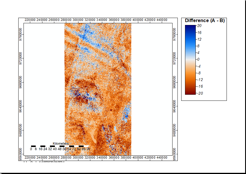Areas in darker red and darker blue indicate higher areas of difference. Areas where the elevation changes dramatcially such as on steep slopes there is more difference in the elecation data. The area shown here has is one such area: looking at the satellite imagery for the same area, we can see that this is an area with a lot of steep valleys: The areas of dark red indicate that the SRTM sampling found higher elevations than the ASTER sampling. The spots of dark blue indicate that the ASTER data had high elevations. The differences in elevation are a result of differences in sampling methods between ASTER and SRTM. ASTER uses stereo correlation while SRTM uses radar interferometry. Being aware of the of the differences in the data helps to idenify where there may be uncertainty in the stream flow anaylsis.

The same tool can be used to run an anaylsis on outputs of flow accumulation from the SRTM and ASTER data. Here are the results of ASTER flow accummulation minus SRTM flow accummulation. This map shows that there is uncertainty spread through the map where both ASTER and STRM in different locations over and under estimated flow accumumulation in comparison to one another. This is shown in the prevalence of both dark red and dark blue. This zoomed in look at the same area where we were looking at difference in the elevation shows how differences in the elevation sampling produce differences in the flow accumulation In this zoom we can also see the error at water bodies where the flow accumulation cannot be accurately sampled because both STRM and ASTER data shows water bodies as flat land.

As this anaylsis shows, there are differences in the flow accummulation depending on the data source used. While it looks more dramatic in the DEM data. the flow accummulation difference results show that there will be differences in the final results that can affect decision making if these outputs are used for real analysis.